Discrete Choice Models - Matlab
Discrete choice models in Matlab
Fork my repo here.
Models available:
- Logit
- Exploded Logit
- Logit with Random Coefficients
- Exploded Logit with Random Coefficients
Discrete choice models are becoming trendier as more data becomes available in multiple areas like health, education, credit markets, and many others. The key idea of them is to model the process of decision making of an individual for choosing a particular option among a discrete set of option, based on individual and option level characteristics. Many applications of this method come to my mind; for instance, estimating the probability of a family choosing where to enroll their children from an array of schools available near their neighborhood, or estimating the probability of choosing a particular mean of transportation for an individual to get to work.
With the objective of estimating these models, I developed dcmLab, a package programed in Matlab, (Python and Julia versions forthcoming) that computes different versions of static discrete choice models that maximize the likelihood, or the joint likelihood, of a decision problem. You can also add non observable heterogeneity to your model by using the random coefficients routine in the package.
In this post I pretend to briefly explain how the code works in the case of a very simple logistic model without unobservable components. For a description of the mathematical details I recommend reading “Discrete choice methods with simulation” by Kenneth Train 2009.
The whole package can be found here The simplest way of testing it is to clone the repository, open matlab and run mainLogit or mainExplodedLogit depending on which model you want to test.
Disclaimer: I know Matlab’s OOP is very slow and defining all the functions within a single class can be computationally inefficient, however, I decided to have all the code in one class anyways to prevent loading the repo with many .m files. If you’re looking for efficiency, I recommend separating the functions in different .m files, I did that for many other projects and it worked 100% guaranteed.
Ok, here we go!
First, the script defines variables entering into the model, in this case we define the nXX different explanatory variables and store them in cell array XX which contains arrays of nObs observations and nOptions options. Our explanatory variables here will be random arrays that comply with the mentioned characteristics but could easily be replaced by characteristics from the real world. All the variables that will be used in the model will be stored in the Data structure.
nObs = 10000; nOptions = 20; nXX = 15;

Data.nObs = nObs;
Data.nOptions = nOptions;

Data.XX = {};
for ii = 1:nXX
    Data.XX{ii} = randn(nObs,nOptions); %Variable 1
end
Second, in order to generate data on choices we have to arrange the coefficients that will enter the routine and define the model type we want to be testing. Our logistic model is Model 1 and will use random parameters for each X variable. After defining the parameters and the XX variables we can generate fake choices conditional on them using dcmLab.generateFakeChoices(parameters, false). This routine uses as inputs a parameter array and a bool that is true if we want to generate the feasible choice set based on a Deferred Acceptance algorithm (the matlab implementation was adapted by Mohit Karnani), or false if we want to define a random feasible choice set. For this tutorial we will opt for the second. The result of the routine is a new element in Data named ChoiceIndex.
Pack.Model = 'Model 1'; %This define the type of model to estimate

parameters = dcmLab.setupParameters();
% 1.5. Generate Choices
dcmLab.generateFakeChoices(parameters, false); %Estimate fake data
After generating choices, we define the utility function we will use dcmLab.utilityFunction(parameters, true) and check whether the gradients for the objective function of the model are correctly defined. What dcmLab.checkGradient(parameters,passedUtilityFunction) does is compute the difference between the analytic gradient and the numerical gradient that should be zero if the gradient is correctly defined.
passedUtilityFunction = @(parameters) dcmLab.utilityFunction(parameters,  true);
dcmLab.checkGradient(parameters,passedUtilityFunction)
Once gradients for all parameters were checked, we continue with the optimization procedure. Basically, we introduce our utility function in a handler again, plus some random initial values for our parameters and pass the function to the optimization routine. dcmLab.estimationNLP uses the quasi-newton optimization method from Matlab to fit parameters. You can play with the method by changing hyperparameters within dcmLab if you consider necessary.
passedUtilityFunction = @(theta) dcmLab.utilityFunction(theta, true);
[theta_quasinewton,fobj1,~,~]=dcmLab.estimationNLP(theta_init, passedUtilityFunction);
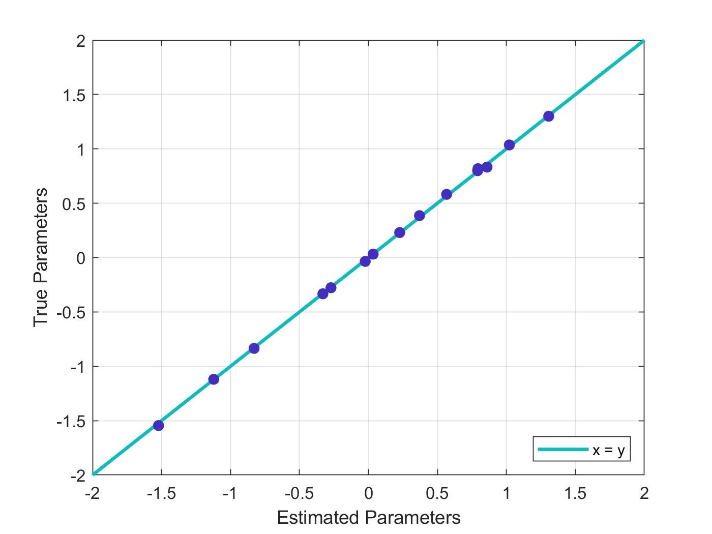
This method should perfectly recover the parameters we used to define ChoiceIndex after convergence is reached. Here is a scatterplot that shows how well our estimated coefficients fit to the true parameters.
In addition to the Matlab optimization method, I also built an stochastic gradient descent procedure with Adam optimizer (Kingma & Ba 2015) that can be faster for optimizing objective functions when the dimensionality of the parameter space and/or the number of observations in the model increases. This procedure uses mini batches of data -instead of the whole sample- to estimate the magnitude and direction where parameters should be updated iteration by iteration based on adaptive estimates of lower-order moments. To visualize performance run the next lines of code.
%4.1. Define batch size:
batchSize = 2^10;
nIter = 120;
%4.2. What happens when we start from the true values?
initial_values = theta_init(1,:); %initial_values = theta_init(s,:);
passedUtilityFunction = @(theta) dcmLab.utilityFunction(theta, true);
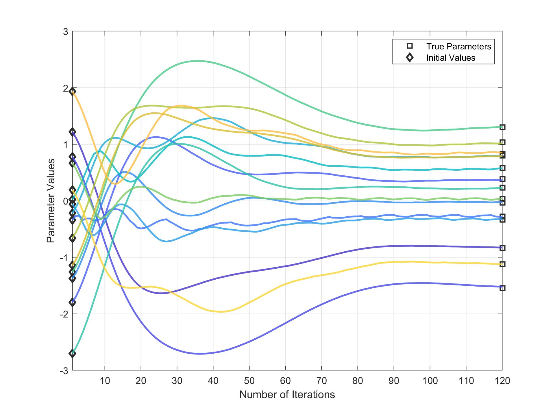
[theta_estimated_Adam, allTheta]= dcmLab.optimizationAlgorithm(initial_values, batchSize, 'Adam', nIter, passedUtilityFunction);
Here we plot how parameters converge after 120 iterations:
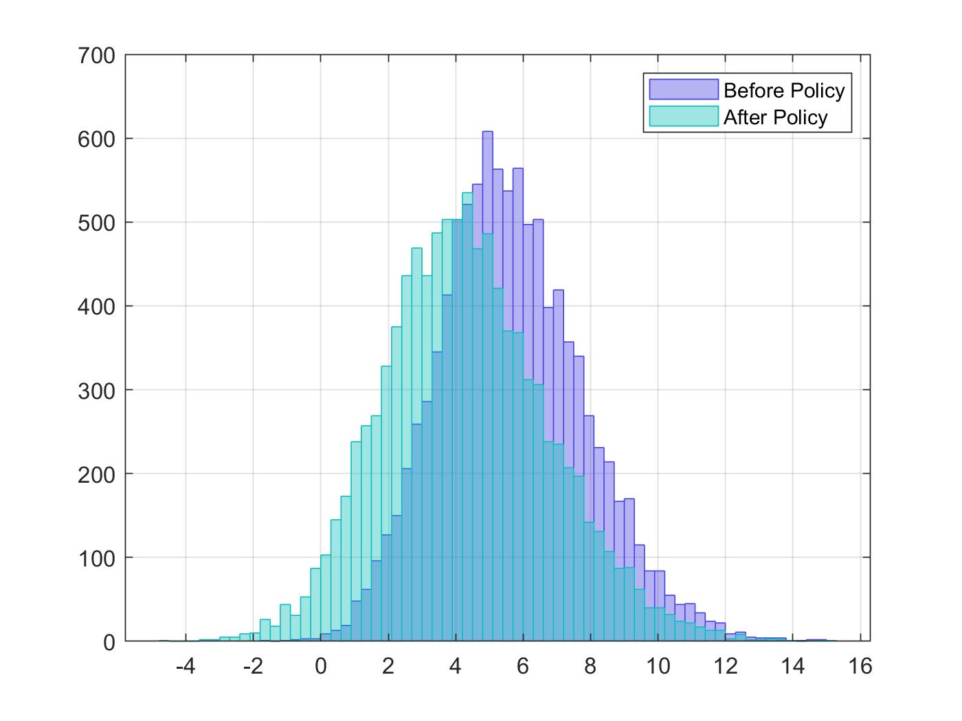
After parameters were recovered, we can make multiple experiments. For instance, here I added code that simulates how utility would change if we reduce the set of options available to individuals, say, closing schools or closing routes where a car can transit to go to a destination.
nKilled = 5;
Policy = ~(Ranking > nOptions - nKilled);
Data.FeasibleSet = logical(double(Data.FeasibleSet).*double(Policy));

utilities1  = dcmLab.simulateUtilities(parameters);
[~,choice1] = max(utilities1,[],2);

histogram(utilities0(bsxfun(@eq, 1:size(utilities0,2), choice0)), 'EdgeColor', CC(10,:), 'FaceColor', CC(10,:), 'FaceAlpha', 0.4)
hold on
histogram(utilities1(bsxfun(@eq, 1:size(utilities1,2), choice1)), 'EdgeColor', CC(50,:), 'FaceColor', CC(50,:), 'FaceAlpha', 0.4)
legend('Before Policy','After Policy')
grid on
box on
Evidently, reducing options can reduce overall utility.
I hope this post was useful to understand dcmLab. Please, if you have any comments or want to make changes to improve dcmLab, don’t hesitate on submitting pull requests to the repo. If your changes are approved I’ll publish my gratitude to your contribution to this post and tweet about it.
Bibliography:
Train, K., & Weeks, M. (2005). Discrete choice models in preference space and willingness-to-pay space. In Applications of simulation methods in environmental and resource economics (pp. 1-16). Springer, Dordrecht.
Kingma, D. P., & Ba, J. (2014). Adam: A method for stochastic optimization. arXiv preprint arXiv:1412.6980.